Appearance
User Posting Trend and Seasonality
tags: Python Seaborn statsmodels
In this section, we analyze the trend and seasonality of users' posting habits.
The number of works posted to the Archive is time-series data, which is a set of obervations obtained in different time periods. We are not going into details of time-series models in this section. Instead, we'll briefly showcase two components of time-series analysis: autocorrelation, and decomposing trend and seasonality from the data set.
Loading File
python
# Load Python library
import pandas as pd

# Load file
path="/home/pi/Downloads/works-20210226.csv"
chunker = pd.read_csv(path, chunksize=10000)
works = pd.concat(chunker, ignore_index=True)
Data Cleaning
Since majority of the works posted to AO3 are in English, we choose English works in the data set for analysis. The data set contains the creation date of each work, and we're going to sum up the number of works posted per month from 2008 to 2021. All of the Python functions used here are discussed in previous blog posts.
python
# Select two columns that we're interested in
# Select English works for analysis
eng = works[['creation date','language']][works['language'] == 'en']

# Drop NA values
eng = eng.dropna()

# Preview of the DataFrame
eng| creation date | language | |
|---|---|---|
| 0 | 2021-02-26 | en |
| 1 | 2021-02-26 | en |
| 2 | 2021-02-26 | en |
| 3 | 2021-02-26 | en |
| 4 | 2021-02-26 | en |
| ... | ... | ... |
| 7269688 | 2008-09-13 | en |
| 7269689 | 2008-09-13 | en |
| 7269690 | 2008-09-13 | en |
| 7269691 | 2008-09-13 | en |
| 7269692 | 2008-09-13 | en |
6587693 rows × 2 columns
python
# Make sure date column is in datetime format
eng['creation date'] = pd.to_datetime(eng['creation date'])

# Group by monthly posting
# Use pd.Grouper because it aggregates throughout the years
eng = eng.groupby([pd.Grouper(key='creation date',freq='1M')]).count()

# Preview of the DataFrame
eng| language | |
|---|---|
| creation date | |
| 2008-09-30 | 928 |
| 2008-10-31 | 480 |
| 2008-11-30 | 337 |
| 2008-12-31 | 239 |
| 2009-01-31 | 499 |
| ... | ... |
| 2020-10-31 | 141120 |
| 2020-11-30 | 122796 |
| 2020-12-31 | 154417 |
| 2021-01-31 | 147813 |
| 2021-02-28 | 137125 |
150 rows × 1 columns
Plotting The Data
Line Plot
python
# Import libraries
# Top line is Jupyter Notebook specific

%matplotlib inline

import matplotlib.pyplot as plt
import seaborn as sns
python
# Line plot using seaborn library
# Orignal data
ax = sns.lineplot(data=eng)

# Aesthetics
ax.set_title('Works Posted Per Month \n 2008-2021')
ax.legend(title='Language', labels=['English'])
plt.ylabel('works')
Text(0, 0.5, 'works')

Seasonal Plot
python
# Add a year column
eng_annual = eng.copy().reset_index()
eng_annual['year'] = eng_annual['creation date'].dt.year

# Rename columns
eng_annual.columns = ['creation date', 'works', 'year']

# Preview data
eng_annual| creation date | works | year | |
|---|---|---|---|
| 0 | 2008-09-30 | 928 | 2008 |
| 1 | 2008-10-31 | 480 | 2008 |
| 2 | 2008-11-30 | 337 | 2008 |
| 3 | 2008-12-31 | 239 | 2008 |
| 4 | 2009-01-31 | 499 | 2009 |
| ... | ... | ... | ... |
| 145 | 2020-10-31 | 141120 | 2020 |
| 146 | 2020-11-30 | 122796 | 2020 |
| 147 | 2020-12-31 | 154417 | 2020 |
| 148 | 2021-01-31 | 147813 | 2021 |
| 149 | 2021-02-28 | 137125 | 2021 |
150 rows × 3 columns
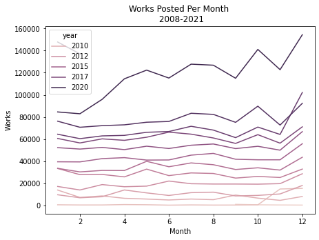
python
# Visualizaion
ax = sns.lineplot(data=eng_annual, x=eng_annual['creation date'].dt.month, y='works', hue='year', ci=None)

# Aethetics
plt.xlabel('Month')
plt.ylabel('Works')
plt.title('Works Posted Per Month \n 2008-2021')
Text(0.5, 1.0, 'Works Posted Per Month \n 2008-2021')
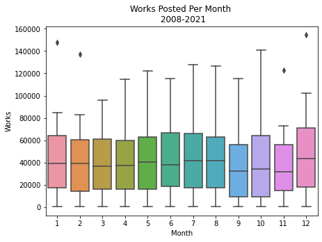
Boxplot Distribution
python
# Monthly Posting
ax = sns.boxplot(data=eng_annual, x=eng_annual['creation date'].dt.month, y='works')

# Aethetics
plt.xlabel('Month')
plt.ylabel('Works')
plt.title('Works Posted Per Month \n 2008-2021')
Text(0.5, 1.0, 'Works Posted Per Month \n 2008-2021')
python
# Annual Posting
ax = sns.boxplot(data=eng_annual, x=eng_annual['creation date'].dt.year, y='works')

# Aethetics
plt.xlabel('Year')
plt.ylabel('Works')
plt.title('Works Posted Per Year \n 2008-2021')
Text(0.5, 1.0, 'Works Posted Per Year \n 2008-2021')

Autocorrelation
Autocorrelation shows the correlation of the data in one period to its occurrence in the previous period. When data are both trended and seasonal, we will see a pattern in our ACF (AutoCorrelation Function) graph.
python
# Import Statsmodels library
import statsmodels.api as sm
python
# AFC plot
ax = sm.graphics.tsa.plot_acf(eng, lags=37)

#Aesthetics
plt.xlabel('Lag')
plt.ylabel('Correlation')
Text(0, 0.5, 'Correlation')
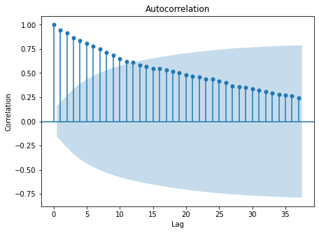
The ACF decreases when the lags increase, indicating that the data is trended.
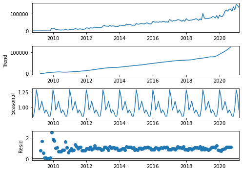
Decomposing A Time Series Data
Time series data comprise three components: trend, seasonality, and residual (noise). An additive decomposition assumes that: data = trend + seasonality + residual; alternatively, a multiplicative decomposition assumes that: data = trend x seasonality x residual.
python
# Import Statsmodels library
from statsmodels.tsa.seasonal import seasonal_decompose

# Adjust figure size
plt.rcParams['figure.figsize'] = [7, 5]
python
# Additive Decomposition
result_add = seasonal_decompose(eng, model='additive')
ax=result_add.plot()
python
# Multiplicative Decomposition
result_mul = seasonal_decompose(eng, model='multiplicative')
ax = result_mul.plot()